ARTIFICIAL NEURAL NETWORKS
0.
Preparation: review of principal
components and PC regression
> attach(USArrests)
> names(USArrests)
[1]
"Murder"
"Assault" "UrbanPop" "Rape"
> states
= row.names # The first column in dataset “USArrests” did not have any name
> pc
= prcomp(USArrests, scale=TRUE)
> biplot(pc)
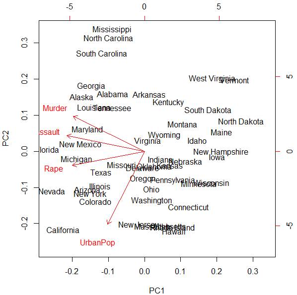
Red vectors are projections of the original X-variables
on the space of the first two principal components. We can see that the first
principal component Z1 mostly represents the combined crime rate,
and the second principal component Z2 mostly represents the level of
urbanization.
1.
Artificial neural network with no
hidden layers is just linear regression
Artificial neural networks are available in
package neuralnet.
> library(neuralnet)
Create the training and testing data.
> attach(Auto)
> n = length(mpg)
> Z = sample(n,200)
> Auto.train
= Auto[Z,]
> Auto.test
= Auto[-Z,]
> nn0 = neuralnet( mpg ~ weight+acceleration+horsepower+cylinders, data=Auto.train, hidden=0 )
> nn0
Error Reached Threshold Steps
1 1720.963134
0.009532195866
8565
> plot(nn0)
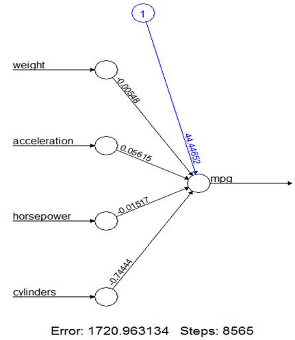
This is the linear regression! Weights are
slopes, and the intercept is shown in blue.
> lm(
mpg ~ weight+acceleration+horsepower+cylinders, data=Auto.train )
Coefficients:
(Intercept) weight acceleration horsepower cylinders
44.446611467 -0.005475864 0.056149012
-0.015172364 -0.744442628
2.
Artificial neural network
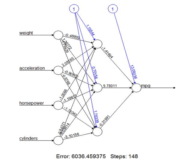
Now, introduce 3 hidden nodes.
> nn3 = neuralnet(
mpg ~ weight+acceleration+horsepower+cylinders, data=Auto.train, hidden=3 )
> plot(nn3)
3.
Prediction power
Which ANN gives a more accurate prediction? Use
the test data for comparison.
> Predict0 = compute(
nn0, subset(Auto.test,
select=c(weight, acceleration, horsepower, cylinders) ) )
This prediction consists of X-variables
“neurons” and predicted Y-variable “net.result”.
> names(Predict0)
[1] "neurons"
"net.result"
> mean(
(Auto.test$mpg - Predict0$net.result)^2 )
[1] 18.83350028
Prediction MSE of this ANN is 18.83.
> Predict3 = compute( nn3, subset(Auto.test,
select=c(weight,acceleration,horsepower,cylinders) )
)
> mean(
(Auto.test$mpg - Predict3$net.result)^2 )
[1] 61.84868054
Its 3-node competitor has a much higher
prediction MSE.
4.
Multilayer structure
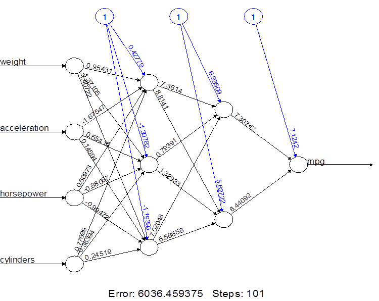
The number of hidden nodes can be given as a
vector. Its components show the number of hidden nodes at each hidden layer.
> nn3.2 = neuralnet(
mpg ~ weight+acceleration+horsepower+cylinders, data=Auto.train, hidden=c(3,2) )
> plot(nn3.2)
5.
Artificial neural network for
classification
> library(nnet)
Prepare our categorical variables ECO and ECO4
> ECO = ifelse( mpg > 22.75, "Economy", "Consuming"
)
> ECO4 = rep("Economy",n)
> ECO4[mpg < 29] = "Good"
> ECO4[mpg < 22.75] =
"OK"
> ECO4[mpg < 17] =
"Consuming"
> Auto.train = Auto[Z,]
> Auto.test = Auto[-Z,]
Train an artificial neural network to classify
cars into “Economy” and “Consuming”.
> nn.class = nnet( as.factor(ECO) ~ weight +
acceleration + horsepower + cylinders, data=Auto.train,
size=3 )
# weights: 19
initial
value 169.471585
final
value 138.379332
converged
> summary(nn.class)
a 4-3-1 network with 19 weights
options were - entropy fitting
b->h1
i1->h1 i2->h1 i3->h1 i4->h1
-0.11 -0.35
0.12 0.32 0.16
b->h2
i1->h2 i2->h2 i3->h2 i4->h2
0.59 -0.37
-0.56 0.67 0.44
b->h3
i1->h3 i2->h3 i3->h3 i4->h3
0.50 0.16
0.41 -0.49 0.02
b->o
h1->o h2->o h3->o
-0.12 -0.27
0.03 0.02
This ANN has p=4 inputs, one layer of M=3 hidden
nodes, and a single (K=1) output. We need to estimate M(p+1)+K(M+1)
= (3)(5)+(1)(4) = 19 weights.
Classification into K > 2 categories is
similar.
> nn.class = nnet( as.factor(ECO4) ~ weight+acceleration+horsepower+cylinders, data=Auto.train, size=3 )
# weights: 31
initial value 333.799856
final value 276.956630
converged
> summary(nn.class)
a 4-3-4 network with 31 weights
options were - softmax
modelling
b->h1 i1->h1 i2->h1 i3->h1 i4->h1
0.39 0.69 -0.58
0.23 0.11
b->h2 i1->h2 i2->h2 i3->h2 i4->h2
-0.49 -0.67 -0.65
-0.68 0.11
b->h3 i1->h3 i2->h3 i3->h3 i4->h3
-0.67
0.24 0.59 0.43
0.00
b->o1 h1->o1 h2->o1 h3->o1
0.98 -0.25 0.32
-0.12
b->o2 h1->o2 h2->o2 h3->o2
0.13 0.41 0.19 -0.02
b->o3 h1->o3 h2->o3 h3->o3
0.20 0.28 0.34 -0.01
b->o4 h1->o4 h2->o4 h3->o4
-0.24 0.42 -0.09 0.41
Here K = 4 categories, so we are estimating (3)(5) + (4)(4) = 31 weights.